This post covers the foundational knowledge of machine learning (ML). The core of ML is built on probabilistic and
statistical modeling, optimization, and linear algebra.
Given the breadth of the topic, I won't cover all aspects exhaustively but will highlight key points extracted from
the following three books
[1,
2,
3]
Make assumptions and build the model (In Stat, it will involve creating parameters and specifying prior
distributions).
Learning (In Stat, referred to as parameter learning and posterior inferences).
Specify a loss function (estimator), e.g., MLE, NLL, MSE
Handle the intractable terms or parameters (e.g., partition function), using approximation or change of
variables.
Solve the loss function with optimization
Inference/testing/prediction
Different names of data and target
Data \(X\): Feature, covariates, predictors
Target \(y\): Label, target, response
Uncertainty of model parameters or prediction: Captured by the distribution variance.
Uncertainty of the prediction: variance of the predictive distribution (softmax)
Uncertainty of the model parameters: variance of the parameter's distribution
Basic Theorems
Curse of dimensionality:
To cover the same fraction of the data space, the number of samples needed increases exponentially as the
dimension increases.
To fit high-D data, other than using a large dataset, we can also make assumptions of the data and build
models with inductive bias (e.g., hierarchical structure).
No free lunch theorem: No single model works well for all problems.
We will need to build different models and conduct model selections.
Well-known trade-offs: Variance and bias, efficiency, model complexity, and generalization, accuracy and
transparency
Ockham's Razor: Always try to choose the simplest model (add regularization).
Task, measure, experience
Tasks: Classification, regression, anomaly detection, clustering, factor analysis \(p(x|z,\theta) =
\mathcal{N}(x|wx+\mu, \sigma)\), classification/regression with missing value (learn joint distributions and
marginal out), synthesis and sampling, imputation of missing values, density estimation
Population risk: \( \mathbb{E}_{x\sim p} [L(f(x))] \).
Structure risk: empirical risk plus regularization.
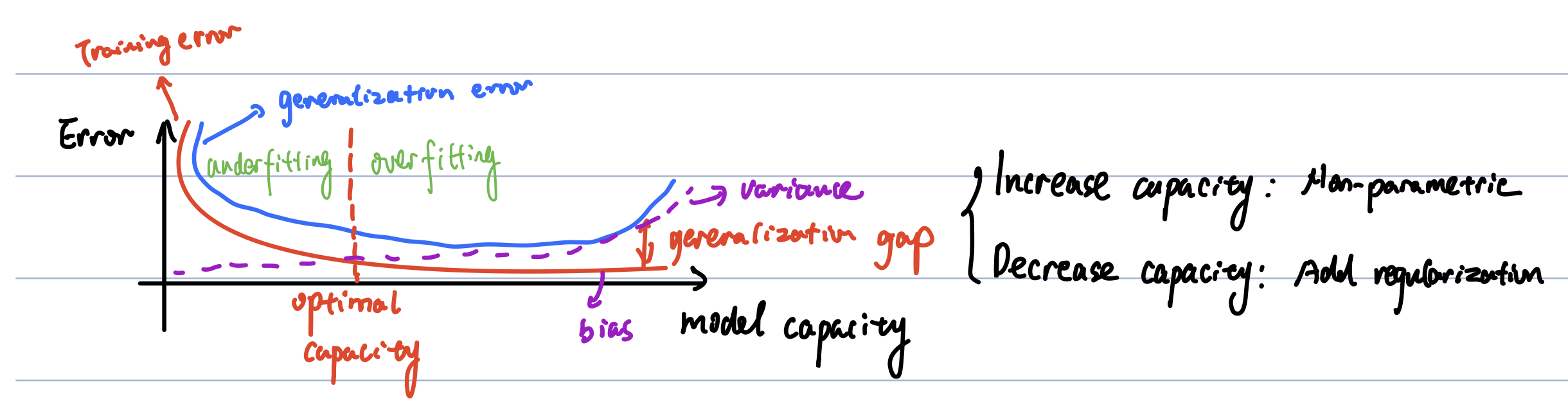
Capacity: model's ability to fit a wide range of functions (commonly also referred to as complexity). Select
different hypothesis spaces to control model capacity.
Errors
Model error: error introduced during model selection, the ability to represent data.
Data error: error introduced during data sampling.
Optimization error: error introduced during learning, the presentation power of the weight.
Bias and variance trade-off. Overfitting means the model has a high training accuracy but performs poorly
on the testing set.
Underfitting means the model has a low training accuracy (undertrained).
The k-NN model is a good example of understanding the tradeoff figure.
When K=1, the model reaches the highest capacity, and the training error is zero; however, the testing error is high
given a testing sample may be far from any training data.
When K=N, the model has the lowest capacity, and the training error and testing error are all high.
Also, consider bias and variance, K=N has the lowest variance and K=1 has the highest variance but the lowest bias.
Double descent: As the model becomes more complex, the testing error may reduce again for a double concave shape.
This is typically observed in deep learning models. The reason for such a phenomenon could be when the model reaches
zero bias,
the model may overfit the noise, shortcuts, and spurious correlations in the training data.
As the model becomes more complex, it will learn causal relationships and become generalizable. This indicates we can
apply over-parameterization when training deep learning models.
Estimation, Bias, variance
The model training process is also referred to as estimation and there are two types of estimation:
point estimation, which finds optimal values for model parameters (typical way of model training );
density estimation, estimate the distribution of model parameters to assess uncertainty (less efficient and rarely
used).
Bias measures the point estimation error. \( bias(\hat{\theta}) = \mathbb{E}(\hat{\theta}) - \theta \).
A good estimator should be unbiased or asymptotically unbiased. Below, we give two examples of how to compute bias.
Mean of Bernoulli distribution: given an estimation of the parameter \( \hat{\theta} = \frac{1}{m}\sum x_i\)
(sample mean), the bias is \( \mathbb{E}[\frac{1}{m}\sum x_i] - \theta = 0 \)
Mean of Gaussian distribution: sample mean is also an unbiased estimation of \(\mu \).
Variance of Gaussian distribution: \(\sigma^2 = \mathbb{E}(x^2) - (\mathbb{E}(x))^2 \). Given an estimation
\(\hat{\sigma}^2 = \frac{1}{m}\sum_{i} (x_i - \hat{\mu})^2\), the bias is as follows:
$$ \mathbb{E}[\hat{\sigma}^2] - \sigma^2 = \frac{1}{m}\sum_{i} (x_i - \hat{u})^2 - \sigma^2 = \frac{m-1}{m} \sigma^2
- \sigma^2 = -\frac{1}{m}\sigma^2$$
\( \sum_i (\frac{x_i-\hat{\mu}}{\sigma}) \sim \mathcal{X}^2_{m-1} \), where \( \mathcal{X}^2_{m-1} \) refers to the
chi-square distribution (sum of the square of the standard Gaussian distribution).
Variance measures the variation of estimation when training data are resampled. There is a trade-off between
variance and bias when MSE is used.
$$ \mathbb{E}[(\hat{\theta}-\theta)^2] = Bias(\hat{\theta})^2 + Var(\hat{\theta}) $$
Consistency stands for \(lim_{m \rightarrow \infty} \hat{\theta}_{m} = \theta\). Two other well-known theorems:
the law of large numbers and the central limit theorem.
MLE and MAP
Maximum likelihood estimation \(\mathbb{E}_{x\sim p_{data}} [\text{log} p_{model}(x;\theta)] \), where
\(p_{data}\) is the empirical distribution.
It can also be derived by minimizing the KL divergence between \(p_{data}\) and \(p_{model}\), where KL divergence is
the typical measurement for distribution difference. Note that KL is asymmetric.
MLE requires the data distribution lies in the model family and it is statistically efficient.
MAP estimation \(\mathbb{E}_{x\sim p_{data}} [\text{log} p_{model}(x;\theta)] + \color{red}{\text{log}
p(\theta)} \),
where \(p(\theta)\) is the prior term. It is equal to regularization terms, when \(\theta\sim \mathcal{N}(0,
\sigma^2)\), it is equal to weight decay.
Limitation of traditional ML (Open-discussion)
The curse of dimensionality, reliance on local consistency and smoothness assumption.
In a high-D space, the number of samples needed to represent each subspace increases exponentially and the local
smoothness assumption may be broken, requiring way more data to represent an entire space.
Deep learning leverages manifold learning and hierarchical structures, where the subspace at each hierarchy can
preserve smoothness or is of a lower dimension.
Independent: \( x \bot y: p(xy)=p(x)p(y)\); \( x \bot y|z: p(x,y|z)=p(x|z)p(y|z)=g(x,z)h(y,z)\)
Bayes' rule: \( p(\theta|D) = \frac{p(D|\theta)p(\theta)}{p(D)} \), e.g., Monty hall problem
Common distributions
Bernoulli (used for classification): logits
\(f(x)=xW^T+b\) or \(\text{log} \frac{p}{1-p}\); sigmoid function \(\frac{1}{1+e^{-f(x)}}\)
Categorical (used for classification):
softmax function \(p_{c} = \frac{e^{a_c}}{\sum_{c'} e^{a_c'}} \). To prevent overflow or underflow, we apply the
log-sum-exp trick.
Gaussian distribution: sum of independent
variables, used to model residual errors. Linear regression: \(p(y|x,w) = \mathcal{N}(xw^T, \sigma^2)\). Dirac delta
function.
Beta distribution (\(0\leq x \leq 1\)) and (inverse) Gamma distribution (\( x>0\)): these two distributions are
used for Bayesian hierarchical modeling; Beta is used to model the parameter of Bernoulli; InverseGamma is used to
model the standard deviation of Gaussian.
Transformation of random variables
Change of variables: \(p_{y}(y) = p_{x}(x)|\text{det}(\frac{dx}{dy})|\); also need to replace x with f(y) in the
pdf (e.g., Gaussian)
Monte Carlo approximation: \(\mathbb{E}[f(x)] \approx \bar{f(x_s)}\); Change of variable and MC method is often
used to estimate the likelihood term (in variational learning),
where we need to sample from an unknown distribution \(p(\theta)\). First, transform \(\theta \) as a function of a
standard Gaussian and then use MC to approximate the likelihood.
Linear transformation, convolutional theorem, and central limit theorem (mean of the iid variable follows a
Gaussian distribution \(\mathcal{N}(\mu, \frac{\sigma^2}{N})\)), the law of large number (applied to sample mean),
Chebyshev's inequality
Joint distributions
Covariance and (Pearson) correlation: \( corr[x,y] \in [-1,1], x\bot y, corr[x,y]=0; y=ax+b, corr[x,y]=1\).
Correlation does not imply causation (spurious correlation). Simpson's paradox: statistical trends appearing in
different groups can disappear or reverse when these groups are combined
Mutual information measures non-linear relationships.
Multivariate Gaussian: computing \(\Sigma^{-1}\) is \(O(D^3)\), Mahalanobis distance, which measures the
geometric shape of the Gaussian PDF (a rotation of Euclidean distance).
Marginal and conditional distributions of MVN.
Dirichlet distribution/process: used to model the parameter of the categorical distribution in
Bayesian/frequentist hierarchical model.
Exponential family: An abstraction form of a set of distributions, with a partition function \(z(x)\),
\(\text{log} z(x)\) is convex because the hessian matrix is non-negative.
When describing a distribution where we know \(\mathbb{E}[f(x)] = F\) and the prior distribution \( q(x) \),
min\(KL(p|q) + \lambda_0(1-\sum_x p(x)) + \lambda_1(F - \sum p(x)f(x))\),
if q is a uniform distribution, p is exponential family (model with the largest entropy).
KL divergence: \(KL(p||q) = \mathbb{E}_{x\sim p(x)}[\text{log}\frac{p(x)}{q(x)}]\). MLE is equal to minimize
\(KL(p_{data}||p_{model})\), where the data distribution is the empirical distribution.
Cross entropy: \(H(p||q) = \mathbb{E}_{x\sim p(x)}[-\text{log}q(x)]\), used for classification loss
Jensen's inequality: \(f(\mathbb{E}[x]) \leq \mathbb{E}[f(x)]\), where \(f(x)\) is convex. Jensen's inequality is
important and is widely used in approximation.
Learning and inference: parameter learning refers to the process of solving model parameters (point estimation);
inference refers to the process of quantifying the uncertainty about an unknown quantity from finite samples.
Bayes' rule: \( p(\theta|D) = \frac{p(D|\theta)p(\theta)}{p(D)} \), where \( p(\theta|D) \) is posterior that can
quantify the uncertainty (prevent overfitting); predictive distribution \(p(y|x,D) = \int p(y|x,D, \theta)
p(\theta|x,D) d\theta\)
Conjugate prior: the prior and posterior follow the same distribution family.
Full Bayesian: \( p(\theta, \phi|D) \propto p(D|\theta) p(\theta|\phi)p(\phi)\).
Bayesian statistics/ML
Model examples: logistic regression, mixture Gaussian model.
Approximation and scale up: compute \(p(\theta|D), p(y|x, \theta)\) in an efficient way. Only in a few cases the
posterior can be computed exactly (e.g., conjugate prior)
Grid approximation: discretize a continuous distribution.
Laplace approximation: Approximate \( p(D|\theta) \) with a multivariate Gaussian, \( p(D|\theta) =
\frac{1}{Z}e^{\epsilon(\theta)} \), where \(\epsilon(\theta) = -\text{log}p(\theta, D)\) is the energy function
and \(Z=p(D)\) is the partition function.
\(p(\theta|D) = \mathcal{N}(\hat{\theta}, H^{-1})\), where \(\hat{\theta}\) is the mode.
Variational approximation (Biased): \(\text{argmin} KL(q(\theta)|p(\theta|D))\). \(q(\theta)\) is the
variational distribution.
MCMC: \(q(\theta) = \frac{1}{s}\sum_s\delta(\theta-\theta_s)\) is the MC approximation of \(p(\theta|D)\).
Sample \(\theta_s \sim p(\theta|D)\) without evaluating \(p(D)\).
Bayesian decision theory: choose the right predictions
Basis: Loss function \(L(H, a)\), where \(H\) and \(a\) represents states and actions.
Posterior expected loss \(R(a|x) = E_{p(h|x)} [L(h,a)]\).
Loss and measurement for classification: zero-one loss (adjust the threshold based on the loss for balancing FP
and FN), precision, recall, F1, false discovery rate (per class accuracy), RoC curves, calibration errors.
Regression losses: \(L_1, L_2\), and Huber loss (combination of \(L_1 \& L_2\) )
Some other related topics: Bayesian hypothesis testing (Bayesian t-test, assume data is fixed and compute
posterior for testing), model selection, cross-validation, information criteria (BIC, AIC)
Frequentist statistics
Basis: Do not treat model parameters as random variables but measure uncertainty by calculating how a quantity
estimated from data
would change if the data changes; Frequentist: data is changing in different trials but parameters are fixed
(Bayesian: data is fixed but parameters are random variables )
Sampling distribution of an estimator (estimate uncertainty):
Estimator: Decision procedure that specifies what actions to take given data \((\theta = \pi(D))\)
Sampling distribution: The distribution of results if we apply the estimator multiple times to different
datasets sampled from the same distribution
\(p(\pi(\tilde{D}))=\theta|\tilde{D}\sim\theta^*) \approx \frac{1}{s}\sum_s\delta(\theta=\pi(D))\), where
\(\theta^*\) is the true distribution and D represents the sampled data
When using MLE as the estimator and the sample size is large, the sampling distribution is Gaussian for some
model
$$ \mathcal{N}(\theta|\theta^*, (NF(\theta^*))^{-1}), F(\theta^*) = E_{p(x|\theta)} [\triangledown \text{log}
p(x|\theta) \triangledown \text{log} p(x|\theta)^{T}] $$
A high Determinant of the Fisher matrix means high log-likelihood curvature, and the sampling distribution has a
low variance (robust to repeated trials).
Bootstrap approximation of the sampling distribution (parametric or non-parametric), Bootstrap is equivalent to
the posterior of a non-informative prior
Confidence interval (Different from credible interval): \(p(L(\tilde{D}) \leq \theta \leq
U(\tilde{D})|\tilde{D}\sim\theta^*) = 1 - \alpha\);
frequentist hypothesis testing (Define the null hypothesis and compute the p-value, i.e., the probability under the
null hypothesis of observing a test)
SVD: \(A = UDV^{T}\), \(AA^{T} = UDD^{T}U^{T}\), can be used for dimension reduction (i.e., remove the part of
the matrix that has a low eigen/singular value)
Other decomposition: LU, QR, Cholesky
Optimization basics
local vs. global optimum; flat local optimum \(L(\theta) \ge L(\theta^*)\); strict local optimum \(L(\theta) >
L(\theta^*)\)
Necessary condition for local optimum: \(f'(\theta) = 0\), Sufficient condition: \(f'(\theta) = 0\) and
\(f''(\theta) \ge 0\) or Hessian is positive definite, saddle points: \(f'(\theta) = 0\) but Hessian can be negative
Constrained and unconstrained optimization: feasible set \(C = \{ \theta: g_{i}(\theta) \ge 0: j \in \mathcal{I};
h_{k}(\theta) = 0 : k \in \varepsilon \}\), \(\text{argmin}_{\theta \in \mathcal{C}} L(\theta) \)
Convex and nonconvex: Convex set: for any \(x, x' \in \mathcal{S}\), \(\lambda x + (1-\lambda) x' \in
\mathcal{S}\); Convex function: for any \(x, y \in \mathcal{S}\) and for any \(0 \leq \lambda \leq 1 \): \(f(\lambda
x + (1-\lambda)y) \leq \lambda f(x) + (1-\lambda)f(y) \); \(f\) is convex if and only if \(f''(x) \ge 0 \) for all
\(x\)
Smooth and nonsmooth: The objective and constraints are continuously differentiable \(|f(x_1) - f(x_2)| \leq
L|x_1 - x_2|\); Nonsmooth: at some points, the gradient is not well defined.
Momentum: \(m_t = \beta m_{t-1} + (1-\beta) g_{t}, \theta_t = \theta_{t-1} - \eta_t m_t\); move faster along the
directions that were previously good; Nesterov momentum
Second-order methods: Newton's method, BFGS (move faster but more costly than first-order)
More advanced methods with momentum and lr changes: AdaGrad, RMSprop, Adam
Constrained optimization: KKT and Lagrange - transform constrained optimization into unconstrained optimization
or Proximal gradient method - take a step in the gradient direction and project the result into a space that
respects the constraints (proximal operator), e.g., projected gradient descent.