This post covers the foundational and advanced topics of multilayer perceptron (MLP), the most basic building block of
all deep learning models, including transformers. The main material I referred to is [1].
Before diving into MLP, I first discuss the insights of why deep learning achieves way better performance than
traditional statistical and ML models. The insights are based on the limitations of traditional models discussed in
[ML basis].
(1) High model capacity: this is the most obvious reason. Deep neural networks by design are easier to scale than
traditional models such as SVM, CRF, HMM, which enables them to learn more complex data and handle more complex
learning tasks (as learnability is proportional to model capacity).
Additionally, deep neural networks support model parallelism, enabling more efficient training when models are large. For
example, tree-based models can also go very large by continuously adding more sub-tree layers. However, they do not support
parallel training, making the computational cost increase quadratically as the model becomes larger.
(2) Recall that traditional ML models rely on the local consistency and smoothness assumption, which is often
invalid in high dimensional spaces. Deep neural networks (DNNs) have a hierarchical structure where the lower layers
learn small subspaces and the higher layers learn the relations and abstractions of different small subspaces.
As a result, DNNs can learn part of subspaces and generalize to others, which enables them to learn and represent
high-D spaces with fewer data samples required. A counterexample is the K-NN classifier, where the relationship
between each K group of samples is not modeled and the model cannot generalize well.
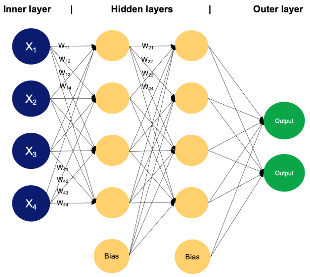
A figure of a fully connected MLP is shown as follows.
Demonstration of the fully connected MLP model [1].
Input: the model takes a vector as the input, i.e., \(x \in \mathbb{R}^{p}\), where p is the input dimension as
well as the number of input neurons (e.g., 4 in the figure above).
Hidden layers
Neuron: the basic element of a neural network, each neuron receives input signals from the connected neurons
in the last layer and gives an output signal to its connected neurons in the next layer.
Each layer has multiple neurons, where the number of neurons is a model hyper-parameter, as well as the number
of layers.
Neurons in DNNs were proposed to conceptually simulate the neurons in human brains. The operation on each neuron
is a linear transformation followed by a non-linear activation function.
The linear transformation is just a regression \(Wx + b \) and the activation function controls whether the
neuron is activated or not, which simulates the neurons in human brains.
Weight: Each neuron is associated with a weight vector \(w \in \mathbb{R}^{d_{l-1}}\), where \(d_{l-1}\) is the
number of neurons in the previous \((l-1)\)-th layer.
Each layer is associated with a weight matrix \(W_l \in \mathbb{R}^{d_{l-1} \times d_{l}} \), where \(d_{l}\) is the
number of neurons in the current \(l\)-th layer.
Bias: Each layer has a bias \(b \in \mathbb{R}^{d_{l}} \), which is the intercept in the linear operation.
Activation (functions): the activation function controls whether the current neuron gives non-zero (activated)
values or zero (saturated) values. The most common activation function is ReLU.
Output layer
Number of neurons: the number of neurons in the output layer is related to the desired task of the neural
network. For example, in classification tasks, the number of neurons is the number of classes.
Activation functions: the activation function is typically softmax in multi-class classification and sigmoid in binary classification.
Forward pass
Forward pass means calculating the output by passing a given input through the entire model. Mathematically, it is
written as
$$ M_l = \text{relu} (M_{l-1}W_{l} + b_{l}), \quad \text{for} \ l= 1, 2, ..., L, \quad
o = \text{softmax}(M_{L} W_{L+1} + b_{L+1}) , $$
where \(L\) is the number of hidden layers, \(M_{l} \in \mathbb{R}^{N \times d_l}\) is the output of the \(l\)-th
layer, \(W_{L+1} \in \mathbb{R}^{d_L \times C}\) and \(b_{L+1} \in \mathbb{R}^{C}\) are the parameters of the output
layer, and \(o\) is the output of the model. \(N\) is the batch size.
Note that here we consider the input as a matrix. In more complex models, the input can have more than one dimension,
the MLP model is applied to the last dimension of the input.
Without the activation function, the model is equivalent to a logistic regression model.
Negative log-likelihood loss \(-\frac{1}{N}\sum_{i}\text{log}\ p(y_i|x_{i}, \Theta)\), where \(p(y_i|x_{i},
\Theta)\) is the model's prediction probability on the true class of the \(i\)-th sample.
Derive the NLL loss from the cross-entropy loss: minimize the cross-entropy between the true label distribution
and the predictive distribution of the model:
$$H(p_{data}, p_{model}) = -\mathbb{E}_{p_{data}}[\text{log}\ p_{model}] = -\frac{1}{N}\sum_{i} \sum_{c}
y_{ic}\,\text{log}\ p(y_i = c \mid x_{i}, \Theta)$$
Here \( p_{data} \) follows the empirical distribution, where the probability mass at the given samples is 1 and 0
elsewhere. \( p_{model} \) is the model's predictive distribution, which follows a categorical distribution with
the parameter \( p(y|x, \Theta) \).
Cross-entropy loss is the general form of the NLL loss. When the label is in one-hot encoding and the softmax
function is used, the cross-entropy loss is the same as the NLL loss.
Derive the NLL loss from the maximum likelihood estimation (MLE): $$ -\mathbb{E}_{p_{data}}[\text{log}\ p(y_i|x_i,
\Theta)] = -\frac{1}{N}\sum_{i} \text{log}\ p(y_{i}|x_{i}, \Theta)$$
Here, \( p_{data} \) is the empirical distribution, and \( p(y_i|x_i, \Theta) \) is the likelihood, which follows a
categorical distribution.
The MSE loss: \(\frac{1}{N}\sum_{i} \| y_i - \hat{y}_i \|_2^{2} \). This loss is widely used in regression
models. It can also be derived from the general MLE loss when the likelihood follows a Gaussian distribution.
The MAE loss: \(\frac{1}{N}\sum_{i} |y_i - \hat{y}_i| \). This loss is also used in regression models. It can
also be derived from the general MLE loss when the likelihood follows a Laplace distribution.
Compared to MSE, MAE loss is robust to outliers and can encourage zero loss when \(y\) has a high dimension. However,
it may not be smooth or differentiable.
The MAP loss: \(\text{log}\ p(\Theta|y,x) = \text{log}\ p(y|\Theta, x) + \text{log}\ p(\Theta) + \text{const}\).
Here \(p(\Theta)\) is the prior distribution, and the \(\text{log}\ p(\Theta)\) term is equivalent to the
regularization term.
When the model output layer is the softmax function, \(\text{log}\ p_{c} = o_c - \text{log}\ \sum_{c'} e^{o_{c'}}\), where
the second term can be computed using the log-sum-exp trick/function.
Backward pass
After computing the loss value, the MLP or any deep learning model can be trained using the backpropagation
algorithm.
Below, we compute the gradient of the loss function with respect to the model parameters using the chain rule in an
MLP model.
Consider an MLP model with \(L\) fully connected layers. The input to this model is \(X \in \mathbb{R}^{n \times p}\)
and each hidden layer has a ReLU activation function.
$$ M_{l} = \text{relu}(M_{l-1}W_{l}^T+b_{l}^{T}), \quad \text{for} \ l=1, 2, ..., L,$$
$$ O = M_{L}W_{L+1}^T+b_{L+1}^{T},$$
$$ P = \text{softmax}(O),$$
where \(M_{l} \in \mathbb{R}^{n \times d_{l}}\) is the output of the \(l\)-th layer and \(d_{l}\) is the hidden
dimension of the \(l\)-th layer.
\(W_{l} \in \mathbb{R}^{d_{l} \times d_{l-1}}\) is the weight matrix and \(b_{l} \in \mathbb{R}^{d_{l}}\) is the
bias of the \(l\)-th layer.
\(P \in \mathbb{R}^{n \times C}\) is the output of the softmax function.
Note that this section uses the convention \(W_l \in \mathbb{R}^{d_l \times d_{l-1}}\) (with a transpose in the forward
pass) for derivation convenience, which is the transpose of the convention used in the architecture section.
We first calculate the gradient of the loss w.r.t. the model output logits \(O\).
We start with a simple case where the batch size is 1, the number of classes is \(3\), and the last hidden dimension
is \(d_L=2\).
Here, \(O = [O_1, O_2, O_3]\), \(P = [P_1, P_2, P_3]\), and assume the true label is \(y = [0, 1, 0]\). The cross-entropy
loss is \(L = -\text{log}(P_2)\).
$$\left(\frac{\partial L}{\partial O}\right)^T = \frac{\partial P}{\partial O} \left(\frac{\partial L}{\partial P}\right)^T,$$
where \(\frac{\partial L}{\partial P} = [0, -\frac{1}{P_2}, 0]\) and \(\frac{\partial P}{\partial O} = \text{diag}(P)
- PP^T\) (the softmax Jacobian, which is symmetric).
As such, $$\left(\frac{\partial L}{\partial O}\right)^T = \begin{bmatrix}
P_1-P_1^2 & -P_1P_2 & -P_1P_3\\
-P_1P_2 & P_2-P_2^2 & -P_2P_3\\
-P_1P_3 & -P_2P_3 & P_3-P_3^2\\
\end{bmatrix}
\begin{bmatrix}
0 \\
-\frac{1}{P_2}\\
0 \\
\end{bmatrix}
=
\begin{bmatrix}
P_1 \\
P_2-1\\
P_3 \\
\end{bmatrix}
,$$
Hence, \(\frac{\partial L}{\partial O} = P - Y \).
Next, we calculate the gradient of the loss w.r.t. the pre-activation of the \(L\)-th hidden layer, \(\hat{M}_{L}\)
(where \(M_L = \text{relu}(\hat{M}_L)\)).
$$
\frac{\partial L}{\partial \hat{M}_{L}} = \frac{\partial L}{\partial O}\,\frac{\partial O}{\partial M_L}\odot
\frac{\partial M_{L}}{\partial \hat{M}_{L}}
$$
where \(\frac{\partial M_{L}}{\partial \hat{M}_{L}} = \mathbf{1}\{\hat{M}_{L} \geq 0\} \in \mathbb{R}^{n \times d_{L}}\)
is an elementwise indicator (so the product with it is a Hadamard product), and
\(\frac{\partial L}{\partial O}\,\frac{\partial O}{\partial M_L} = \frac{\partial L}{\partial O}\, W_{L+1}\). Here
the calculation process is similar to the process of calculating \(\frac{\partial L}{\partial W_{L+1}}\).
The rest of the gradients can be backpropagated using the chain rule. The gradients of the loss w.r.t. the early layer
pre-activations have a similar form to \(\frac{\partial L}{\partial \hat{M}_{L}}\), and the gradients of the loss
w.r.t. the early layer parameters have a similar form to \(\frac{\partial L}{\partial W_{L+1}}\).
As we can observe from the equations above, each gradient is represented as a matrix calculation, where the batch size
can be generalized to more than one.
More specifically, the general gradients are as follows:
The model is trained using a certain gradient descent algorithm with the gradient calculated above. Below, we list
some common training algorithms:
Gradient descent: $$W_{l}^{t+1} = W_{l}^{t} - \lambda \frac{\partial L}{\partial W_l^{t}},$$
where \(\lambda\) is the learning rate. It controls the learning process's convergence speed and whether it is stable.
An overly large learning rate will lead to oscillation around the optimal point, and an overly small learning rate
will lead to slow convergence.
Gradient descent: update the model using the gradients of all data samples.
Stochastic gradient descent: update the model using the gradient of every data sample.
Mini-batch stochastic gradient descent: update the model using the gradients of a batch of data samples.
Learning rate scheduling: automatically adjust the learning rate during training, starting with a large one and
decaying linearly or according to a cosine function.
Momentum SGD: \(v_{t+1} = \beta v_t + (1-\beta)\frac{\partial L}{\partial W_l^{t}}\), \(W_{t+1} = W_t - \lambda v_{t+1}\).
This enables smooth parameter updates and avoids being affected by extremely large gradients (gradient clipping can also be used).
Adam (Adaptive Moment Estimation): (1) adaptive learning rates
(smaller gradient magnitudes have a larger lr); (2) combines first and second moments;
(3) bias correction: normalize the moments (moving average) to avoid bias towards zero at the initial stage; (4)
robust to sparse gradients because of (1), (2), and (3).
Variations of Adam: the original Adam by default has \(\ell_2\)-norm weight decay, which is not optimal for large-scale
transformer learning (cannot adjust regularization strengths, which is suboptimal for transformer models that are
sensitive to regularization). AdamW, which decouples weight decay from Adam, is preferred.
During testing, we fix the model parameters and evaluate the model's performance on the test set. Typically, we assume
the testing and training data have the same distribution (IID assumption).
However, when the testing data has a different distribution or its distribution shifts over time, it will cause an OOD issue
or a concept drift issue. We may discuss these issues in later posts.
Below, we summarize the widely used metrics for evaluating the model's performance:
Accuracy: \(\frac{\text{Num. of correctly classified samples}}{\text{Num. of total samples}}\). Accuracy can be
problematic when classes are imbalanced.
Precision, recall, F1: calculated for each class, they better reflect the model's performance on each class than
accuracy.
Precision = \(\frac{TP}{TP+FP}\), which reflects the model's false positive rate. Precision is critical for anomaly
detection models.
Recall = \(\frac{TP}{TP+FN}\), which reflects the model's performance on samples belonging to the current class.
Note that balanced accuracy is the average recall across all classes.
F1 score = \(\frac{2\,\text{precision}\cdot\text{recall}}{\text{precision}+\text{recall}}\).
ROC and AUC: ROC shows the model's TPR (recall) and FPR under different thresholds, where random guessing lies on the
diagonal. AUC \(\in [0,1]\) is the area under the ROC curve. It represents the likelihood that the model ranks a
randomly chosen positive instance higher than a randomly chosen negative instance. The higher the AUC, the better
the model.
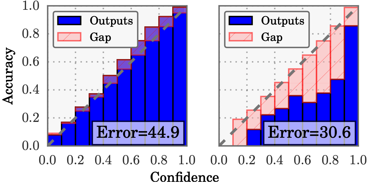
Average calibration error (ACE): evaluates how well a model's
predicted probabilities match the true probabilities. For example, if the model gives an 80% confidence for a class,
a perfectly calibrated model should correctly predict 80% of data from that class.
The figures below show the calibration curve of a model (taken from the original ACE paper). The x-axis is the
average prediction probability/confidence and the y-axis is the accuracy. The diagonal line is the perfect
calibration line. The ACE is the area between the red and the blue part.
ACE is calculated by dividing the samples into different bins based on their prediction probabilities and computing
the average difference between their accuracy and confidence in each bin:
\(\frac{1}{M}\sum_i|\text{acc}(i)-\text{conf}(i)|\).
Demonstrations of overconfident and underconfident models reflected by ACE. [2]
Overconfidence does not always mean the model is overfitting. It is more about how much the model trusts its
prediction and will also affect the user's trust in the model. Resolving the overconfidence or underconfidence issue
can be done with temperature/Platt scaling.
Sometimes, the ACE will have a very high variance across different training epochs due to bin sensitivity, bin
sample imbalance, etc. We can use the ECE (Expected Calibration Error), which is a weighted average of the per-bin
calibration gap (weighted by the number of samples in each bin), or we can use dynamic bins and unbiased sampling
(even distribution of samples in each bin and weight classes and bins properly).
Regularizations are widely used to prevent overfitting and improve model generalizability.
Most of the regularization methods constrain the model's capacity.
From the Bayesian perspective, regularization is equivalent to adding a prior distribution to the model parameters
\(\text{log}\ p(\Theta)\).
Below, we list some widely used regularization methods:
Parameter norms: weight decay, i.e., the \(\ell_2\)-norm penalty, which is equivalent to adding a Gaussian prior on the
model parameters, may not work well for large models.
The \(\ell_1\)-norm penalty is equivalent to adding a Laplace prior on the model parameters, which encourages sparsity.
In linear regression models, these are called ridge and lasso. The regularization that combines \(\ell_1\) and \(\ell_2\) is
called elastic net.
Dataset augmentation: this refers to a broader group of methods that try to enlarge the diversity of the training
set to improve model generalizability. It is useful when the original training data are biasedly sampled.
Some common data augmentation methods include adding random noises, linear interpolation, augmentation based on
explanations, and adversarial samples.
Dropout: Drop certain neurons during training to reduce the model capacity. During testing, simulate the average
case by multiplying model parameters with the dropout probability. This is, from my personal experience, the
most general regularization method in many use cases.
Other methods: early stopping, bagging, parameter sharing.
Distributed computing is critical and necessary for training large models.
Although it is not very often used to train MLP models, it is still valuable to study the parallel training for MLP
given their simple architectures.
The popular parallelism methods include data parallelism, data + model parallelism, pipeline parallelism, and tensor
parallelism.
In distributed computing, each node means each computer.
Each worker means each process, it can have one or multiple GPUs.
In total, the number of workers should be smaller than the number of nodes * number of GPUs per node.
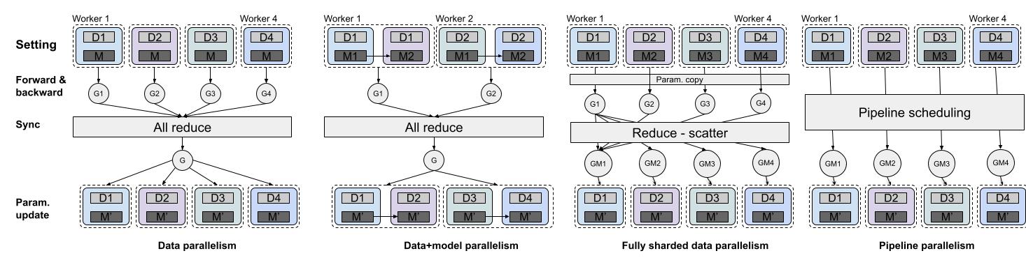
Data parallelism (DDP)
This method copies the same model to multiple workers (GPUs) and each worker processes a different batch of data.
Each worker has a copy of the model and optimizer state and calculates the forward pass and gradients based on its
local data.
The gradients are synced via ``all_reduce'' before the model is updated.
The widely used synchronization methods include bulk synchronous parallel (sync when all gradients are calculated;
inefficient but avoids using stale weights) and
asynchronous parallel (efficient but uses stale weights).
Gradient accumulation is a middle-ground approach that syncs the gradients after every K iterations.
The challenges of data parallelism include:
1) it cannot handle large models that exceed the memory of one GPU;
2) the communication and synchronization overhead.
PyTorch's DDP package is the most widely used package for data parallelism.
Data + model parallelism
This method first splits the data into different parts and each part is processed by a specific worker.
Each worker has multiple GPUs and each GPU processes a different part of the model.
The most straightforward way is to split the model into different subsets of layers, where each GPU processes a subset.
This method has lower memory usage than pure data parallelism; however, it introduces more communication overhead.
It may also be slower, given that the data is split into fewer chunks and the later part of the model will need to
wait until the earlier part finishes computing (bubbles).
Another method for data + model parallelism is fully sharded data parallelism (FSDP).
It divides the model into different shards and each shard is assigned to a different GPU.
Each GPU will gather the model parameters from all other GPUs and compute the forward pass and the gradient with the
data assigned to it.
During the backward pass, the gradients of each shard are sent to the corresponding GPU and the optimizer updates the
parameters (two steps: reduce-scatter).
It differs from DDP and DDP with model parallelism in that the model and optimizer states do not need to be copied
to each worker.
Although each process needs to gather the model parameters from all GPUs at some point, it does not need to store the
entire model and optimizer states on each GPU at all times, which is more memory efficient but requires more
communication.
As such, this method is more memory efficient but less time efficient than DDP and model parallelism.
In many cases, the memory and time cost is a trade-off.
Pipeline parallelism
Pipeline parallelism (PP) combines model parallelism with data parallelism to improve efficiency.
It splits model parameters and a minibatch of data at the same time and assigns one model chunk with one data chunk to
one worker.
As such, it enables multiple workers to work at the same time, which reduces the waiting time.
Some popular PP frameworks include GPipe,
PipeDream, and Variations of PipeDream.
Demonstrations of different parallelism methods. Di and Mi means different data and model partitions.
Gi is the gradient computed from the i-th worker and GMi is the gradient of the i-th model partitions. This post
provides a comparison between DDP, FSDP, and PP.
Other memory saving methods
Activation recomputation: only save the activations that need to be shared across workers and recompute the other
activations during backward passes, introducing extra computational overhead but reducing memory cost.
Reduce model size: mixed precision training, quantization, or parameter compression.
Data encoding to compress the intermediate results after the forward passes and decode them back for
back-propagation.
Because of momentum, the optimizer is also memory consuming. For example, Adam stores first and second moment
estimates, requiring \(2\times\) the parameter memory in addition to the parameters themselves. Memory-efficient
optimizers that enable parallelism for optimizer states can help.
Tensor parallelism
Tensor parallelism splits model weights into different tensors and each sub-tensor is assigned to one worker for
forward and backward passes.
Below, we consider two basic methods of splitting the model weights:
Row split
Given a one-layer MLP model with the input \(X \in \mathbb{R}^{n \times p}\).
The model is \( O = XW^T+b^{T}\), \(P = \text{softmax}(O)\), where \(O, P \in \mathbb{R}^{n \times C}\), \(W \in
\mathbb{R}^{C \times p}\) and \(b \in \mathbb{R}^{C}\).
Suppose we divide the weight and bias into \(K\) shards based on the row dimension, i.e., \(W = [W_1, W_2, \ldots, W_K]\),
\(b = [b_1, b_2, \ldots, b_K]\),
where \(W_k \in \mathbb{R}^{C/K \times p}\) and \(b_k \in \mathbb{R}^{C/K}\).
During the forward pass, the output of each shard is \(O_k = XW_k^T+b_k^{T}\), \(O_k \in \mathbb{R}^{n \times C/K}\).
The final output is the column-wise concatenation of all \(O_k\).
During the backward pass, the gradients of the loss w.r.t. \(W_k\) and \(b_k\) are
$$
\frac{\partial L}{\partial W_k} = \left(\frac{\partial L}{\partial O_k}\right)^T X = (P-Y)_{:,\,kC/K:(k+1)C/K}^T X,
$$
$$
\frac{\partial L}{\partial b_k} = \left(\frac{\partial L}{\partial O_k}\right)^T [1,\ldots,1]^T = (P-Y)_{:,\,kC/K:(k+1)C/K}^T
[1,\ldots,1]^T.
$$
Column split
Given a one-layer MLP model with the input \(X \in \mathbb{R}^{n \times p}\).
The model is \( O = XW^T+b^{T}\), \(P = \text{softmax}(O)\), where \(O, P \in \mathbb{R}^{n \times C}\), \(W \in
\mathbb{R}^{C \times p}\) and \(b \in \mathbb{R}^{C}\).
Suppose we divide the weight into \(K\) shards based on the column dimension, i.e., \(W = [W_1, W_2, \ldots, W_K]\),
where \(W_k \in \mathbb{R}^{C \times p/K}\). Correspondingly, the input is split as
\(X = [X_1, X_2, \ldots, X_K]\) with \(X_k \in \mathbb{R}^{n \times p/K}\). The bias \(b\) is not split and is added only once.
During the forward pass, the partial output of each shard is \(O_k = X_k W_k^T\), \(O_k \in \mathbb{R}^{n \times C}\).
The final output is \(O = \sum_k O_k + b^T\).
During the backward pass, the gradient of the loss w.r.t. \(W_k\) is
$$
\frac{\partial L}{\partial W_k} = \left(\frac{\partial L}{\partial O_k}\right)^T X_k = (P-Y)^T X_{:,\,kp/K:(k+1)p/K},
$$
where \(\frac{\partial O}{\partial O_k} = \frac{\partial \sum_k O_{k}}{\partial O_k} = 1\), so
\(\frac{\partial L}{\partial O_k} = \frac{\partial L}{\partial O} = P-Y\).
The forward and backward rules of these two methods can be generalized to multi-layer models and they can also be
mixed together, i.e., some layers are row split and some layers are column split.
The forward pass is straightforward.
For the backward pass, we can first find the gradient of the loss to this layer's output and then calculate the
gradient of the weights based on the row/column split rules above.
Normalizations/standardizations: input normalization/standardization or batch normalization.
Regularizations: weight decay, dropout, etc.
Data augmentation: improve the model's generalizability, noise and adversarial robustness. See the regularization
section for specific methods.
Weight initializations (Xavier and He initialization) and residual connections (especially useful for deep
networks).
LR scheduling, early stopping, and gradient clipping.
Handle class imbalance: upsampling, data augmentation, assigning different weights to different classes when
computing the loss.
Handle noisy labels: use soft labels, mixup, meta-learning, etc. (can write a post specifically about this).
Handle categorical features: use an embedding layer to turn the discrete categorical features into continuous
values.
Debugging: analyze the training/testing loss curves to spot over-fitting and unstable learning (regularization);
check gradients to see if they have weird values, e.g., NaN (normalization and clipping can help);
check model weights and outputs to see if the model collapses (batch norm is an efficient way to address model
collapse).
@article{guo2024mlbasis,
  title   = {Everything you need to know about MLP},
  author  = {Guo, Wenbo},
  journal = {henrygwb.github.io},
  year    = {2024},
  url     = {https://henrygwb.github.io/posts/ml_basis.htm}
}