This post covers the foundations and advanced research topics of transformers and large models.
Transformers were first introduced to conduct machine translations and demonstrated better performance than RNNs and
LSTMs, which were the dominant models for sequential data.
The self-attention mechanism allows transformers to capture long-term input dependencies. Its model depth is
pre-specified and does not change as the input length changes.
As such, transformers do not suffer the gradient vanishing/exploding problem of RNNs and LSTMs.
Later, the encoder of transformers was used for unsupervised pre-training, which serves as a foundation model for many
downstream NLP classification tasks.
Given that transformers can easily scale to large models by adding more layers and more attention heads, their
architecture naturally supports parallelism and distributed computing.
It is easy to scale transformers to very large models and train them on large unlabeled datasets.
Models with high capacity can generalize better and thus become the dominant models in many NLP tasks.
Transformers were also generalized to image domains and other domains with specific tokenization methods, making
them suitable for handling different types of data (multi-modal).
Another line of work trains decoders of transformers as the foundation model for generative tasks. The training task
is more difficult than masked language modeling (MLM) used in pretraining encoders and thus gives models with stronger
generation capabilities.
This forms the foundation of today's LLMs.
As shown in the figure, the transformer model has an encoder-decoder
structure that is composed of multiple transformer blocks, where each block has self-attention, layer
normalization, and fully connected layers.
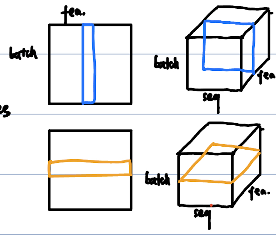
In NLP tasks, the model takes as input a batch of text sequences, \(X_s \in \mathbb{N}^{B \times S_x}\), where \(B\) is the batch
size and \(S_x\) is the maximum sequence length.
The input is first tokenized into a sequence of tokens denoted as \(X \in \{0,1\}^{B \times S \times |V|}\), where \(S\) is the
maximum tokenized sequence length and \(|V|\) is the vocabulary size.
Note that \(S\) may not always be equal to \(S_x\) during tokenization, as each input word may be divided into multiple
tokens. Each token is represented as a one-hot vector of size \(|V|\).
Before feeding the input to the model, the token representations first need to be transformed into a continuous space
to support gradient computation.
This step is called embedding; it is done by multiplying \(X\) with a learnable embedding matrix
\(W_e \in \mathbb{R}^{|V| \times d}\), where \(d\) is the embedding dimension.
The output embedding is denoted as \(E \in \mathbb{R}^{B \times S \times d}\).
The figure below shows the architecture of the transformer model.
Below, we break down the transformer block.
Multi-head attention
Attention was originally introduced in the context of seq2seq models for machine translation [2].
Given an input \(E\) of size \(B \times S \times d\), the original additive attention first computes the attention weights
\(\alpha = \text{softmax}(f(E)) \in \mathbb{R}^{B \times S}\), then calculates the output as \(O = \sum_{j=1}^{S}
\alpha_{:,j}\odot E_{:,j,:} \in \mathbb{R}^{B \times d}\).
This attention introduces a set of parameters in the linear layer \(f\).
In transformers, the dot-product attention is used, which does not introduce additional parameters. It defines a
query matrix \(Q\), a key matrix \(K\), and a value matrix \(V\).
The attention weights are calculated by \(\alpha = \text{softmax}(QK^T/\sqrt{d_h})\), which computes the similarity between keys
and queries.
Then, the output is a weighted sum \(O = \alpha V\). The attention weights control the importance of each value in the
output. They help the model focus on the most relevant information, filtering out noise and irrelevant information.
As such, the model can handle long inputs and capture global long-term dependencies.
Multi-head scaled self-attention.
As shown in the figure above, the attention mechanism takes the same input for calculating queries, keys, and values.
This is called self-attention.
In addition, to encourage the model to learn different hidden correlations of the input, transformers use multi-head
attention, where in each head, the input is first transformed into a unique subspace and then dot-product
attention is computed in each subspace.
Suppose we have \(h\) attention heads; the hidden dimension of each head is \(d_h = d/h\).
The input is first transformed into \(Q_i, K_i, V_i \in \mathbb{R}^{B \times S \times d_h}\) for each head \(i\):
\(Q_i = E W_{Qi}\), \(K_i = E W_{Ki}\), \(V_i = E W_{Vi}\), where \(W_{Qi}, W_{Ki}, W_{Vi} \in \mathbb{R}^{d \times d_h}\) are learnable
parameters.
The output of each head is calculated as \(O_i = \text{softmax}(Q_i K_i^T/\sqrt{d_h}) V_i\).
The final output of the multi-head attention is the concatenation of all heads, \(O_a = [O_1, O_2, \ldots, O_h] W_o\),
where \(W_o \in \mathbb{R}^{d \times d}\) is a learnable parameter.
The dot product is scaled by \(1/\sqrt{d_h}\) to avoid large values entering the softmax function.
We notice that the output dimension is the same as the input dimension, and varying the number of attention
heads does not change the total number of model parameters.
Layer norm and residual connection
The output of the attention is then added to the input and passed through a layer normalization.
\(O+E\) is called a residual connection, which was first introduced in ResNet for image classification.
The residual connection enables the model to learn from identity functions and also makes training easier (avoiding
degradation and gradient vanishing), especially for deep networks.
Layer normalization is calculated for each position in the sequence, so it is not affected much by padding.
In comparison, batch normalization is calculated for each feature across the batch, which will be affected if the inputs are
padded heavily.
Demonstration of the difference between layer norm (top) and batch norm (bottom).
Linear layers
The output of layer normalization is then passed through two linear layers.
$$ \text{FFN}(O_l) = \text{ReLU}(O_l W_1 + b_1) W_2 + b_2. $$
The dimensions of the weight matrices are \(W_1 \in \mathbb{R}^{d \times d_{ff}}\) and
\(W_2 \in \mathbb{R}^{d_{ff} \times d}\), where \(d_{ff} = 4d\) is pre-specified.
The output is again of the same dimension as the input and is passed to the next transformer block.
The main hyper-parameters of the model are the number of layers and the number of attention heads.
Decoder
As shown in the figure, the decoder has three differences from the encoder.
First, the self-attention connected to the input is masked to prevent the model from looking into the future,
which is also called causal attention.
For example, if the model takes as input a sentence "I am a student at UCSB", the model should not use the word
"UCSB" to predict the word "student".
That is, when predicting the word "student", the attention weights corresponding to "at UCSB" are masked out.
Second, the decoder has an additional attention layer that takes the output of the encoder as key and value.
Finally, the model has an additional classification head that predicts the next token in the sequence, which is
modeled as a classification problem with \(|V|\) classes.
This design makes learning more efficient and easier than directly outputting the token embedding, given that
classification problems are discrete and have a smaller space than regression problems.
BERT: Bidirectional Encoder Representations from Transformers
BERT model is a classical variant of the original transformer model.
It was widely used for learning hidden representations for input text and demonstrated better performance than other
language models, like RNN.
The key technique points of this model are as follows:
Each input is composed of two sub-sentences, where an additional <CLS> token is added at the beginning of the
input and a <SEP> token is added in between the two sub-sentences.
An example is <CLS> <I> <AM> <SEP> <LA> <IS> <PAD>, where <PAD> is a padding token.
Each input is associated with a token embedding, a position embedding, and a segment embedding indicating which
sub-sentence the token belongs to.
The model only has the encoder of the original transformer model, which outputs a hidden representation for each
input token.
The learning process has two stages: pre-training and fine-tuning/post-training. The pre-training has two loss
functions:
(1) masked language modeling (MLM), where a certain percentage of the input tokens are masked (replaced with <MASK>)
and the learning objective is to recover the masked tokens.
This is done by adding a classification head to the hidden representation of each masked token.
This objective function forces the model to learn common knowledge about the correlations of input tokens.
(2) Next sentence prediction, which leverages the hidden representation of the <CLS> token to predict whether the two
sub-sentences come from the same source document.
This objective function helps the model learn a holistic representation of the entire input using the <CLS>
token.
The overall objective function can be written as:
$$ \sum_{i\in\mathcal{M}} -\log P(\mathbf{x}_i \mid \mathbf{X}_{\setminus\mathcal{M}}, \Theta)
+ \text{CE}\!\left(y(\mathbf{s}_i,\mathbf{s}_j),\,\hat{y}(\mathbf{s}_i,\mathbf{s}_j; \Theta)\right) $$
where \(\mathcal{M}\) is the index set of the masked tokens, \(\hat{y}(\mathbf{s}_i,\mathbf{s}_j; \Theta) \in \{0,1\}\)
is the model's NSP prediction, and "CE" means the cross-entropy loss.
The fine-tuning for a classification task is to add a classification head (linear probing) to the <CLS> token
representation and conduct a sentence-level prediction.
BERT is good for classification tasks as it can learn hidden correlations in the input, and <CLS> provides a
holistic representation of the entire input.
There are some variants of the BERT model with changes in the embedding layer or tokenization, such as RoBERTa.
Two common model variants are BERT-base (12 layers, 110M parameters) and BERT-large (24 layers, 340M parameters).
This line of models cannot perform generative tasks well because the encoder can access future tokens during
training and the models are not large enough.
GPT: Generative Pre-trained Transformer
GPT models are another line of variants of the original transformer model.
The key differences between GPT and BERT are
1) GPT leverages the decoder of the transformer while BERT uses the encoder;
2) GPT is trained to predict unseen tokens while BERT mainly relies on MLM.
The GPT training tasks are more difficult but once the model is well-trained, it has better generative capabilities
than BERT models.
Also, GPT models typically have a much larger number of parameters than BERT models, such that these models have
enough capacity to handle their difficult training tasks.
GPT models are the foundation of modern LLMs. The most classical papers on GPT models are
GPT-1 proposes the GPT model.
GPT-2
demonstrates scaling up the model can significantly improve the performance.
GPT-3 first proposes testing-phase prompting techniques.
The key technique points of this model are as follows:
Given an input sentence such as <I> <AM> <a> <UCSB> <Gauthier> <EOS>,
where <EOS> is the end token, the tokens will be iteratively fed to the model:
the first input will just be <I>, the second input will be <I> <AM>, and so on. This is equivalent
to masking the later tokens in the input, which is also how it is realized in the implementation.
The tokenization and embedding methods are similar to BERT, but there is no segment embedding. There are
some advanced positional embeddings, which we will discuss later.
The model only has the decoder of the original transformer model. The key here is the causal attention in each
attention block. Also, given that the model does not have an encoder, it will not receive K and V from the encoder.
So the model will again have only one multi-head attention in each block.
The learning process still has two stages: pre-training and fine-tuning. The pre-training only has one loss
function:
autoregressive next token prediction, which iteratively predicts the next token in the input sequence based on the
input \(\mathbf{X}\) and previously generated tokens \( \mathbf{x}'_{1}, \ldots, \mathbf{x}'_{i-1}\).
The model after pre-training can already generate coherent text, the fine-tuning in GPT was originally proposed
to conduct alignment, which trains the model to align with human intentions, such as not generating harmful content,
etc.
Two widely used methods are supervised fine-tuning (SFT) and reinforcement learning from human feedback (RLHF). We
will introduce these methods later.
More recent works also propose different fine-tuning methods to improve the model's capability in specific tasks as
well as its reasoning capabilities.
Testing: the simplest testing method is to just give the model an instruction (could be a question) and ask the
model to generate following the instruction. More advanced works propose a number of techniques to construct the
input such that the model can better understand the input and follow the instructions. We will discuss these
prompting techniques later as well.
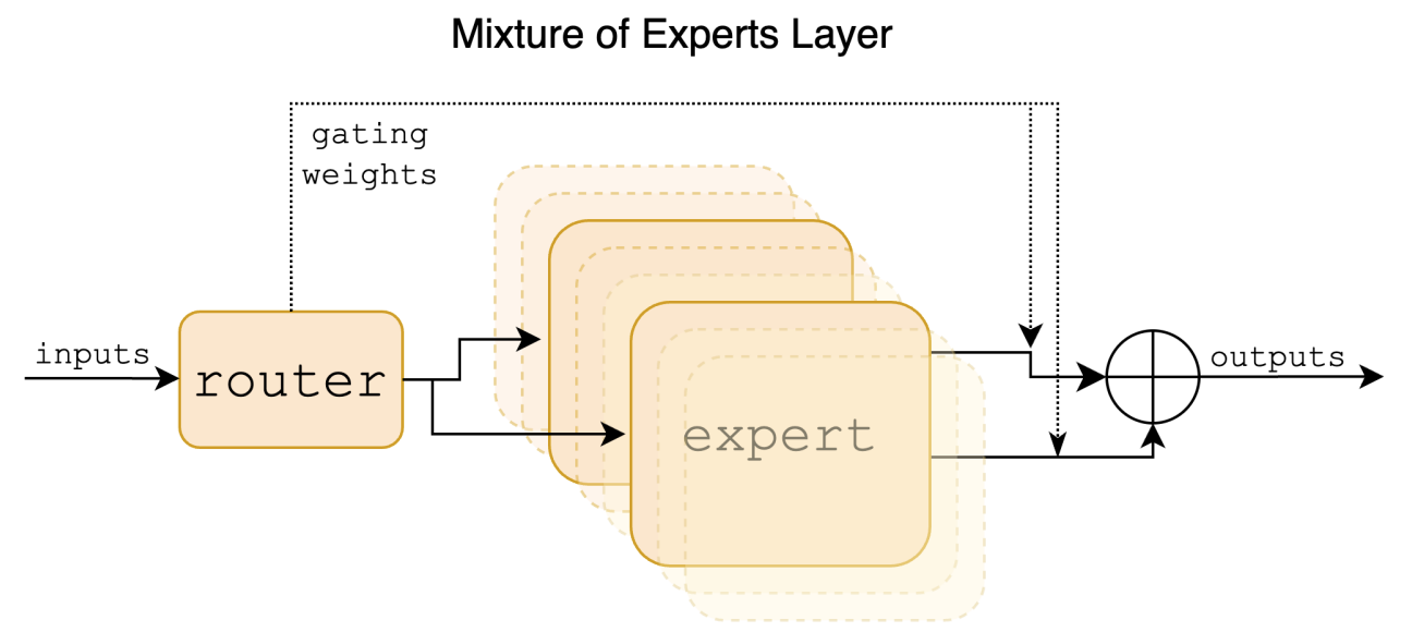
MoE: Mixture of Experts
MoE is a recently emerging model structure that shows better performance than the vanilla GPT models.
The idea stems from the observation that different parts of a large model can be more specialized for certain data or
applications.
Motivated by this observation, MoE was proposed to combine multiple smaller models and test if they can beat a single
large model.
Exploration started with mixing the fully-connected layers in CNNs or RNNs and extended to the entire attention block.
The most recent success of MoE is the DeepSeek-V3 model,
which shows better performance than SOTA large models at a much lower training cost.
Early MoEs.
Mixture of feedforward layers. Design a gating network and \(n\)
experts, where each expert is a feedforward net:
\(y = \sum_i G(x)_i E_i(x)\), where \(G(x)\) is the gating network. It proposes two gating nets, simple softmax
gating and noisy Top-K gating.
The noisy Top-K gating also enables sparse selection, since only the top-K elements in \(G(x)\) will be
non-zero.
Another key point of this method is to add a balance regularization to the loss that encourages all experts to
receive similar utilization, which avoids self-reinforcement.
GShard and Switch
Transformer are early MoEs for transformer models.
They also apply MoE to the final feedforward layers in transformer blocks. The noisy Top-K gating and balance
regularization are applied as well.
Mistral MoEs. The MoE models from Mistral work well on certain tasks, especially the Mixtral-8x7B model.
The model uses a sparse attention mechanism (grouped-query attention and sliding window attention), which we will
introduce later when talking about different attention variations.
Its MoE follows a sparse gating mechanism without adding noise: \(y = \sum_i G(x)_i E_i(x)\), \(G(x) =
\text{softmax}(\text{TopK}(xW_g))\). \(E_i(x)\) is a SwiGLU (Swish-Gated Linear Unit) expert; the FFN in each
transformer block is replaced with SwiGLU.
Basically, they still mix the final linear layers in a transformer block.
Demonstration of the MoE mechanism in the Mixtral model. Router is the gate. [2]
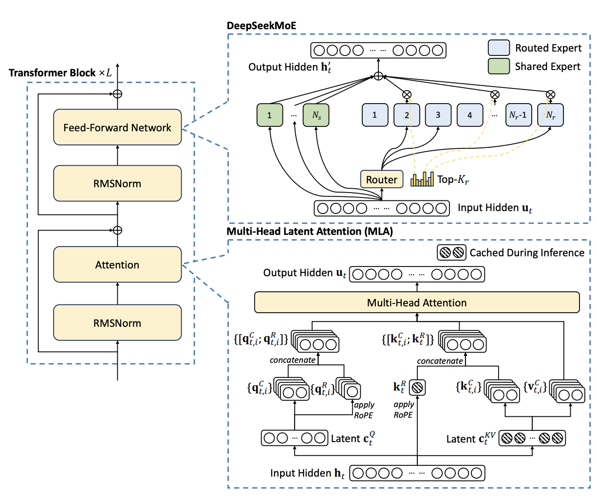
DeepSeek MoEs. DeepSeek's latest model, DeepSeek-V3, also uses
an MoE structure for its feedforward network.
Its key idea is to use finer-grained experts and isolate some experts as shared ones. Given the FFN input (attention
output) of a certain token \(u \in \mathbb{R}^{p}\),
it sets up a total of \(N_s+N_r\) FFNs. The output is \(u + \sum_{s=1}^{N_s} F_s^{(s)}(u) + \sum_{i=1}^{N_r} g_i\,
F_{i}^{(r)}(u)\).
The gating network \(g\) is similar to the top-K sparse gating introduced above. The only difference is that, instead of
computing \(xW_g\), DeepSeek computes \(\text{Sigmoid}(u^T e_i)\), where \(e_i\) is the centroid vector.
The sigmoid is newly added in DeepSeek-V3 and may help with numerical stability.
Demonstration of the DeepSeek-V3 model structure [3]. The
MLA will be introduced later.
This part discusses the optimizations over the vanilla transformer which have been used as SOTA methods.
We will focus on tokenizer, positional embedding, and attention.
Note that MoE can also be taken as an optimization over the FFN in the transformer block.
Tokenizer
SOTA: Byte pair encoding: Start with the smallest tokens and
iteratively merge tokens to form new tokens based on their occurrence in the dataset.
This approach can reduce the number of OOV (out of vocabulary) tokens, which is critical for model performance.
Other tokenization methods: WordPiece/SentencePiece/unigram language model.
Unigram language model: start with all possible sub-word units (single characters and substrings up to a certain
length);
each sub-word is assigned a probability based on frequency;
use the EM method to update the tokenizer to maximize the likelihood.
For some non-common data types, we need to design a specific tokenization method.
The principle is to find a proper vocabulary size. A small size will result in many OOV tokens in the input,
while a large size will end up with a high input dimension (making learning harder).
For multi-modal input, we need to combine multiple tokenizers for different data modalities.
Here is an example of tokenizing blockchain transactions, which
involves hash values
(smart contract function calls, wallet addresses), data values (transaction amount), and text (function log).
Positional embedding
Absolute/fixed positional embedding: use deterministic sine and cosine functions of varying frequencies to encode
positions.
$$PE(p, 2i) = \sin\!\left(\frac{p}{10000^{2i/d}}\right),\quad PE(p, 2i+1) = \cos\!\left(\frac{p}{10000^{2i/d}}\right)$$
where \(p\) is the current position and \(i\) indexes the embedding dimension.
The positional embedding has the same dimension as the token embedding.
Sine and cosine functions are used because they are periodic (can capture repeated patterns) and smooth (so
gradients can be computed).
Each dimension defines a sine or cosine function; lower dimensions have a higher frequency and capture more
fine-grained patterns.
The reason for not using higher frequencies for higher dimensions is to ensure numerical stability.
Fixed positional embeddings do not handle cases where test-time inputs are longer than the training inputs very well.
RoPE: a relative positional embedding method
that can handle flexible sequence lengths and exhibits long-term decay (relative distances are increased for
long-distance token pairs).
Instead of adding positional embeddings to token embeddings, RoPE rotates the projected query and key vectors
by an angle that depends on the token's position index.
Given an input token embedding \(E_i \in \mathbb{R}^{d}\), fixed positional embedding first computes a positional
embedding \(E_i^{p} \in \mathbb{R}^{d}\),
adds them together as \(E_i + E_i^{p}\), and multiplies the result with the Q/K/V weight matrices,
\((E_i+E_i^{p})W_{Q/K/V}\), to get the Q/K/V for the attention.
RoPE instead defines a rotation matrix \(R(\theta, p)\) and computes the input to the attention as
\(R(\theta, p)\,(E_i W_{Q/K/V})\), i.e., the rotation is applied to the projected query/key vectors.
There is a line of research on extending the positional embedding of a pre-trained model during fine-tuning or
inference
[1 (RoPE+Adjusted Base Frequency),
2 (RoPE+Positional interpolation),
3].
They perform position interpolation or extrapolation. As pre-trained models can already take much longer sequences,
these methods draw less attention.
Attention
Below, we introduce some techniques to improve the efficiency of computing attentions during training and testing.
Grouped-query attention (GQA): groups multiple query heads to share the same key/value heads, which reduces the
KV cache size and the K/V projection cost during decoding,
allowing for larger batch sizes and higher throughput. With \(g\) groups, the K/V cache and projection cost are
reduced by a factor of \(h/g\), where \(h\) is the number of query heads.
This method loses fine-grained attention specificity between query heads, resulting in block-like structures in the
effective attention weight matrix \(QK^T\).
Sliding window attention: use partial context to compute the attention; the context length is constrained by a
window size.
The context window is applied to Q, K, and V at the same time. The computational cost is \(O(n w)\), where
\(n\) is the sequence length and \(w\) is the window size.
Shift-short attention: combines grouped-query (short) attention with an inter-group (shift) attention (local
and global attention).
Attention in Mixtral: sliding window attention + grouped-query attention.
Attention in DeepSeek: Multi-Head Latent Attention (MLA). It first maps the input into a low-dimensional latent space and then
maps it back to the original dimension when computing K/Q/V representations.
This helps reduce the memory cost of the KV cache, as only the low-dimensional latent representations need to be
preserved.
Another point is that it breaks down the Q and K representations into two parts: one with RoPE, one without. This is
different from the original RoPE attention where the
rotation is applied to all dimensions. Typical RoPE has \(Q = R(\theta)\,(E W_{Q})\); DeepSeek has \(Q = [R(\theta)\,(E_1 W_{Q}^{(1)}),\ E_2 W_{Q}^{(2)}]\),
where the input is split into a RoPE part and a non-RoPE part.
The detailed computation can be found here.
Here, we go over the widely used pre-training and fine-tuning methods in GPT models.
We will also demonstrate the backward pass of the transformer model.
Data is the first important factor in both pre-training and fine-tuning.
Early works aim to collect high-quality data from the wild. They train another model to filter out low-quality samples.
However, data is like ``fossil fuel'': less and less fresh, untouched data can be found.
More recent work explores how to use LLMs to generate data for continued training.
Pretraining
As discussed above, the pretraining objective function is the next-token prediction loss.
The model iteratively predicts the next token based on the input and the previously generated tokens.
The objective function is written as:
\(\sum_{i=2}^{T} \text{CE}(f(\mathbf{X}, \mathbf{x}'_{1}, \ldots, \mathbf{x}'_{i-1}; \Theta), \mathbf{x}_i)\),
where \(\text{CE}\) represents the cross-entropy loss.
In other words, generating every token is equivalent to conducting a \(|V|\)-class classification.
MoE models typically add an expert balance loss to prevent routing collapse.
Fine-tuning
Supervised fine-tuning (SFT): Apply supervised learning for fine-tuning; basically the loss function is the same
as the pre-training.
RLHF: first, collect human-annotated data and train a reward model.
Then, apply RL to maximize the total reward collected during token generation.
Mapping this to a typical RL setting: state: currently generated tokens \(\mathbf{X}, \mathbf{x}'_{1}, \ldots,
\mathbf{x}'_{i-1}\);
action: generate each token; reward is given by the reward function after each generation.
The training loss function of the reward model is: \(-\log \sigma(R(y_w) - R(y_l))\),
where \(y_w\) and \(y_l\) are the preferred and dispreferred responses. The reward model is trained to assign a higher
reward to preferred responses.
Once we have the reward function, we can apply the PPO loss to
conduct the RL training,
which guarantees a monotonic increase of the total reward.
DPO: direct learning from the preference data without training a
reward model.
The loss function is: \(-\mathbb{E}_{(x, y_w, y_l)\sim \mathcal{D}}\!\left[\log \sigma\!\left(\beta\log
\frac{\pi_{\theta}(y_w|x)}{\pi_{\text{ref}}(y_w|x)} - \beta\log \frac{\pi_{\theta}(y_l|x)}{\pi_{\text{ref}}(y_l|x)}\right)\right]\),
where \(\sigma\) is the logistic sigmoid function, \(\pi_{\theta}\) is the current policy, and \(\pi_{\text{ref}}\) is the reference (base) policy.
More recent research proposes some RL fine-tuning methods to improve the reasoning capability of the model. We
can discuss them in a separate post later.
Backward pass
Similar to the analysis in the MLP post, we compute the
backward pass of a simple transformer model to demonstrate the process.
Consider a decoder-only transformer model with one transformer block. The input embedding is \(E \in \mathbb{R}^{S
\times d}\). Suppose the model has \(h\) attention heads and the hidden dimension of each head is \(d_h = d/h\).
Note that this section uses the convention \(W_{Qi}, W_{Ki}, W_{Vi} \in \mathbb{R}^{d_h \times d}\)
(with a transpose in the forward pass) for derivation convenience, which is the transpose of the convention used in
the architecture section.
The forward pass of the model is:
$$ Q_i = E W_{Qi}^T,\quad K_i = E W_{Ki}^T,\quad V_i = E W_{Vi}^T, $$
$$ O_i = \text{softmax}\!\left(\frac{Q_iK_i^T}{\sqrt{d_h}} + M\right) V_i, $$
$$ O_a = [O_1, O_2, \ldots, O_h] W_o, $$
$$ O_l = \text{LayerNorm}(O_a + E), $$
$$ \text{FFN}_{\text{out}} = \text{ReLU}(O_lW_1^T+b_1)W_2^T+b_2, $$
$$ O = \text{FFN}_{\text{out}} W_{\text{cls}}^T,\quad P = \text{softmax}(O_{S,:}), $$
where \(M\) is the additive causal mask (\(0\) on allowed positions and \(-\infty\) on masked positions),
\(W_{\text{cls}} \in \mathbb{R}^{|V| \times d}\) is the classification head, and \(P \in \mathbb{R}^{|V|}\).
The final loss for predicting the next token is the cross-entropy loss: \(L = -\log P_j\), where \(j\) is the index
of the true next token.
Now, we compute the backward pass. First, we compute the backward pass of the classification head and the feedforward
layers, which is essentially the same as in the MLP model.
The gradient w.r.t. the logits is non-zero only at the last position \(S\):
\(\left(\frac{\partial L}{\partial O}\right)_{i,:} = \mathbf{0}\) for \(i < S\), and
\(\left(\frac{\partial L}{\partial O}\right)_{S,:} = P - Y\), where \(Y \in \mathbb{R}^{|V|}\) is the one-hot
vector of the true token.
Then, we compute the gradient for the attention layer. Note that the attention operation itself does not introduce any
parameters, so we mainly compute the gradients for the layer normalization layer and the linear transformations of each
attention head.
Note that we can ignore the residual connection when computing these gradients within the block, but it will contribute
additively to the gradient for the input embedding.
Here, we first need to handle the layer normalization, which normalizes the input along the last dimension
(feature).
$$ \mu_i = \frac{1}{d}\sum_{j=1}^{d} (O_a)_{ij},\quad \sigma_i^2 = \frac{1}{d} \sum_{j=1}^{d}\left((O_a)_{ij} - \mu_i\right)^2, $$
$$ (\hat{O}_a)_{ij} = \frac{(O_a)_{ij} - \mu_i}{\sqrt{\sigma_i^2+\epsilon}},\quad (O_l)_{ij} = \gamma_j (\hat{O}_a)_{ij} + \beta_j. $$
Let \(g_{ij} \equiv \frac{\partial L}{\partial (\hat{O}_a)_{ij}} = \frac{\partial L}{\partial (O_l)_{ij}}\,\gamma_j\).
The gradients are as follows.
With the gradient for the layer normalization input, \(\frac{\partial L}{\partial O_a}\), we can compute the gradients for
the linear transformations in each attention head.
Recall that \(O_a = [O_1, O_2, \ldots, O_h] W_o\), so
There are four major parallelism mechanisms: data parallelism, model parallelism, pipeline parallelism, and tensor parallelism.
Data parallelism splits the data and assigns different chunks to different devices; it copies the full model to all
devices and synchronizes the gradients calculated on each data chunk.
This approach cannot deal with large models that do not fit on a single device.
Model parallelism splits the model and assigns different parts to different devices. Vanilla model parallelism cannot
fully utilize the computation power of each device because the earlier/later layers need to wait when computing the
later/earlier layers.
We can see that there is a trade-off between memory and speed in data and model parallelism.
Pipeline parallelism splits the model and data into different parts (and the training into different stages) and assigns
different stages to different devices.
There are different pipeline parallelism strategies, all of which try to strike a balance in the memory–speed trade-off.
My earlier post on MLP has a more detailed discussion of these
three parallelism mechanisms.
Tensor parallelism works at a lower level: it divides the model weights into different parts and assigns different parts
to different devices.
The MLP post discusses the forward/backward pass under tensor
parallelism for the MLP model, which is also an essential component of transformers.
Here, we discuss tensor parallelism for the attention module in the transformer model.
Case 1: each attention head is assigned to a different device. The forward/backward pass is as discussed above.
Case 2: we divide \(K\) and \(Q\) in one attention head further into \(N\) shards along the feature dimension,
where each shard has dimension \(S \times d_h/N\).
We keep \(V\) at its original dimension. In this case, the forward pass becomes \(A = \sum_n A_n = \sum_n
Q_n K_n^T\).
The backward pass is similar to the process introduced above, with the key step
\(\frac{\partial L}{\partial A_n} = \frac{\partial L}{\partial A}\,\frac{\partial A}{\partial A_n} =
\frac{\partial L}{\partial A}\).
Case 3: we divide \(K\) and \(Q\) further into \(N\) shards along the sequence dimension, where each shard has
dimension \(S/N \times d_h\).
We keep \(V\) at its original dimension. The forward result \(A = QK^T\) becomes a block matrix made up of
\(N\times N\) sub-blocks, where the \((m,n)\) sub-block is \(Q_m K_n^T\).
The backward pass is also similar, with the key step
\(\frac{\partial L}{\partial (Q_m K_n^T)} = \left(\frac{\partial L}{\partial A}\right)_{mS/N:(m+1)S/N,\,nS/N:(n+1)S/N}\);
that is, we extract the corresponding sub-block of \(\frac{\partial L}{\partial A}\).
Case 4: we divide \(V\) along the feature dimension and keep \(S\). The forward pass produces a column-wise
concatenation of each shard \(O_n\); the backward pass is
\(\frac{\partial L}{\partial V_n} = S^T \frac{\partial L}{\partial O_n}\), where
\(\frac{\partial L}{\partial O_n}\) is the corresponding column shard of \(\frac{\partial L}{\partial O}\).
LoRA
LoRA is an efficient fine-tuning method that learns a task-specific
weight update \(\Delta\Phi\).
\(\Delta\Phi\) adds a weight \(\Delta W = BA\) to each weight \(W \in \mathbb{R}^{d\times k}\), where \(B \in
\mathbb{R}^{d\times r}\) and \(A \in \mathbb{R}^{r\times k}\)
have a low rank \(r \ll \min(d, k)\). When fine-tuning, the model only needs to learn the low-rank matrices \(B\)
and \(A\) under a given objective function. Follow-up works proposed
Q-LoRA, which combines quantization with LoRA, and LongLoRA, which
combines LoRA with RoPE and position interpolation.
In LLMs, inference refers to the process of generating responses based on the input (in probabilistic models,
inference means computing posterior distributions of hidden variables).
Recent research has proposed a number of prompting techniques. Below, we briefly discuss some of the most representative
methods. For a complete list, please refer to the Prompting
Guide.
Instruction generation: the simplest inference method; give the model an instruction and ask the model to generate
following the instruction.
Few-shot examples: a method proposed in GPT-3; feed the LLM a few
examples of the given instruction, which has been shown to help the model better understand the instruction.
Especially useful when we want the model to generate outputs following a specific format.
Chain of Thoughts: ask the model to generate its reasoning process
using instructions like "Please think step by step"; can add few-shot examples of reasoning chains; recent reasoning
models fine-tune the model with CoT trajectories to improve the model's reasoning capability; Self-consistency (majority vote over reasoning chains) further improves
the CoT stability.
Decomposes the reasoning into multiple thought steps, generates multiple thoughts per step, and creates a tree
structure.
Use BFS or DFS and majority vote at each step to get the final output.
BFS uses a queue (FIFO) to manage the nodes to process; DFS uses a stack (LIFO) to manage the nodes to
process.
The idea has also been used in training reasoning models (Monte Carlo Tree Search-based Process Reward Model
training).
ReAct and Reflexion:
combine reasoning with taking actions in the physical world; early-stage LLM-based agents.
Retrieval-augmented generation (RAG): provide LLMs with additional context by retrieving related information from
an external database; the LLM decides what to retrieve, based on embedding-space distances or edit
distances.
Besides the representative methods introduced above, which use human-discovered heuristics for prompt design, there
is another line of work that aims to automatically generate prompts.
Such methods are also used for LLM red-teaming, which generates adversarial prompts targeting different attack goals.
See this post for more details.
White-box methods: assume access to the target LLM; given an input instruction, they leverage the gradient
information to generate prompts; prefix learning is a representative method.
Black-box methods: these methods mostly leverage another helper LLM to generate the prompt for a target LLM; this
problem is equivalent to a black-box search problem in the prompt space, where genetic methods, evolutionary
strategies, and RL can help.
Fuzzing-based methods: Design some mutators using the helper LLM and follow the program fuzzing framework to
mutate an initial prompt based on mutators (e.g., GPTFUZZER); can
further train an RL agent for more efficient mutator scheduling (i.e., RLBreaker)
Fine-tuning-based methods: Directly fine-tune the helper LLM to generate prompts for the target LLM given a
goal; RL is typically used where we define a reward function based on the goal and treat the target LLM as part of
the environment; train the helper LLM accordingly (e.g., RLPrompt
and TEMPERA)
This part introduces three widely used techniques for efficient inference in LLMs: KV cache, quantization, and efficient
decoding.
KV cache is used during autoregressive generation; it stores the key and value for the previously generated
tokens.
Recall that the attention weights are computed as \(qK^T\), where \(q \in \mathbb{R}^{1\times d}\) is the query for the
current token and \(K \in \mathbb{R}^{t \times d}\) contains the keys for the current and previous tokens.
The KV cache stores the key and value for the previous tokens, so that they only need to be calculated once.
$$ q_t = E_tW_{Q},\ k_t = E_tW_{K},\ v_t = E_tW_{V},\ K = [k_{1:t-1};\,k_t],\ V = [v_{1:t-1};\,v_t],\ o =
\text{softmax}(q_t K^T)\,V,$$
where \(o \in \mathbb{R}^{1 \times d}\). When implementing the KV cache, we can use a dictionary to store \(K\)
and \(V\) and update it in the forward function of the model class.
Quantization is the process of reducing the precision of the model weights and activations, which can reduce the
memory and computation cost.
The default precision is 32-bit floating point, which can be reduced to 16-bit floating point or even 8-bit integer.
Quantization: \(q = \text{round}(x/s) + z\), where \(s = \frac{x_{\max}-x_{\min}}{q_{\max}-q_{\min}}\) and
\(z = q_{\min} - \text{round}(x_{\min}/s)\).
Dequantization: \(x = s(q-z)\).
Quantization can be done during training (quantization-aware training) or after training
(post-training quantization).
The most common efficient decoding method is speculative decoding. When conducting inference for a target model, it
uses a small model to generate the candidates for next token and uses the target model to verify the candidates.
The process is called drafting and verification. Drafting with a small model can be faster than directly generating
from the large model and the verification can be done in parallel.
This survey has a comprehensive summary of different drafting and
verification techniques.
Setting a length limit for the generated tokens is also a common practice to reduce the computation cost.
Recent work proposes diffusion LLMs, which leverage the diffusion
process for autoregressive generation and have been shown to be very efficient.
@article{guo2024mlbasis,
  title   = {Transformers: basis and advanced topics},
  author  = {Guo, Wenbo},
  journal = {henrygwb.github.io},
  year    = {2024},
  url     = {https://henrygwb.github.io/posts/ml_basis.htm}
}